API and Documentation

Data Subsampling

Running algorithms which require the full data set for each update can be expensive when the data is large. In order to scale inferences, we can do data subsampling, i.e., update inference using only a subsample of data at a time.

(Note that only certain algorithms support data subsampling such as MAP, KLqp, and SGLD. Also, below we illustrate data subsampling for hierarchical models; for models with only global variables such as Bayesian neural networks, a simpler solution exists: see the batch training tutorial.)

Subgraphs

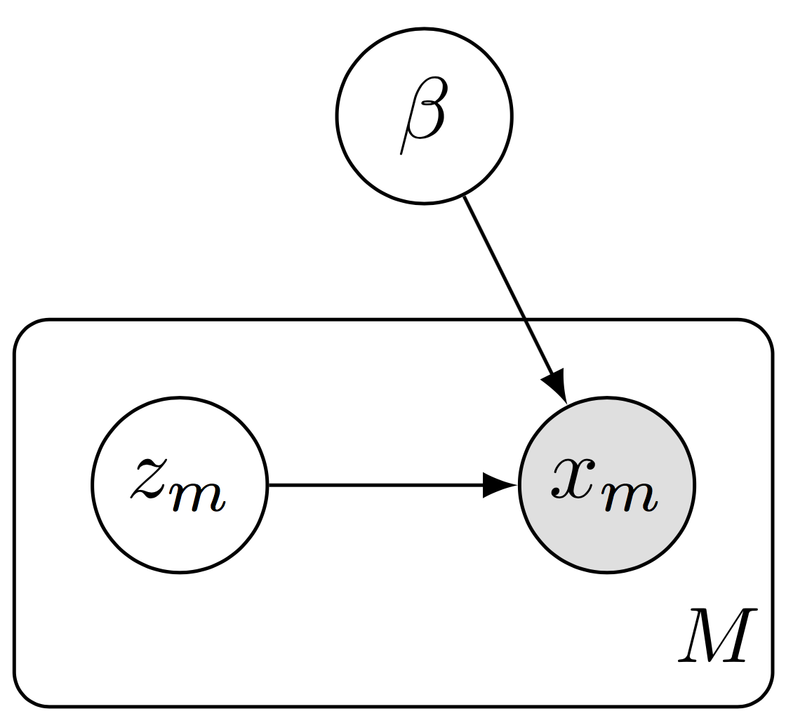
Data subsampling with a hierarchical model. We define a subgraph of the full model, forming a plate of size \(M\) rather than \(N\).

In the subgraph setting, we do data subsampling while working with a subgraph of the full model. This setting is necessary when the data and model do not fit in memory. It is scalable in that both the algorithm’s computational complexity (per iteration) and memory complexity are independent of the data set size.

As illustration, consider a hierarchical model, \[p(\mathbf{x}, \mathbf{z}, \beta) = p(\beta) \prod_{n=1}^N p(z_n \mid \beta) p(x_n \mid z_n, \beta),\] where there are latent variables \(z_n\) for each data point \(x_n\) (local variables) and latent variables \(\beta\) which are shared across data points (global variables).

To avoid memory issues, we work on only a subgraph of the model, \[p(\mathbf{x}, \mathbf{z}, \beta) = p(\beta) \prod_{m=1}^M p(z_m \mid \beta) p(x_m \mid z_m, \beta).\] More concretely, we might define a mixture of Gaussians over \(D\)-dimensional data \(\{x_n\}\in\mathbb{R}^{N\times D}\). There are \(K\) latent cluster means \(\{\beta_k\}\in\mathbb{R}^{K\times D}\) and a membership assignment \(z_n\in\{0,\ldots,K-1\}\) for each data point \(x_n\).

from edward.models import Categorical, Normal

N = 10000000  # data set size
M = 128  # minibatch size
D = 2  # data dimensionality
K = 5  # number of clusters

beta = Normal(loc=tf.zeros([K, D]), scale=tf.ones([K, D]))
z = Categorical(logits=tf.zeros([M, K]))
x = Normal(loc=tf.gather(beta, z), scale=tf.ones([M, D]))

For inference, the variational model follows the same factorization as the posterior, \[q(\mathbf{z}, \beta) = q(\beta; \lambda) \prod_{n=1}^N q(z_n \mid \beta; \gamma_n),\] parameterized by \(\{\lambda, \{\gamma_n\}\}\). Again, we work on only a subgraph of the model, \[q(\mathbf{z}, \beta) = q(\beta; \lambda) \prod_{m=1}^M q(z_m \mid \beta; \gamma_m).\] parameterized by \(\{\lambda, \{\gamma_m\}\}\). Importantly, only \(M\) parameters are stored in memory for \(\{\gamma_m\}\) rather than \(N\).

qbeta = Normal(loc=tf.Variable(tf.zeros([K, D])),
               scale=tf.nn.softplus(tf.Variable(tf.zeros[K, D])))
qz_variables = tf.Variable(tf.zeros([M, K]))
qz = Categorical(logits=qz_variables)

For illustration, we perform inference with KLqp, a variational method that minimizes the divergence measure \(\text{KL}(q\| p)\).

We instantiate two algorithms: a global inference over \(\beta\) given the subset of \(\mathbf{z}\) and a local inference over the subset of \(\mathbf{z}\) given \(\beta\). We also pass in a TensorFlow placeholder x_ph for the data, so we can change the data at each step. (Alternatively, batch tensors can be used.)

x_ph = tf.placeholder(tf.float32, [M])
inference_global = ed.KLqp({beta: qbeta}, data={x: x_ph, z: qz})
inference_local = ed.KLqp({z: qz}, data={x: x_ph, beta: qbeta})

We initialize the algorithms with the scale argument, so that computation on z and x will be scaled appropriately. This enables unbiased estimates for stochastic gradients.

inference_global.initialize(scale={x: float(N) / M, z: float(N) / M})
inference_local.initialize(scale={x: float(N) / M, z: float(N) / M})

Conceptually, the scale argument represents scaling for each random variable’s plate, as if we had seen that random variable \(N/M\) as many times.

We now run inference, assuming there is a next_batch function which provides the next batch of data.

qz_init = tf.initialize_variables([qz_variables])
for _ in range(1000):
  x_batch = next_batch(size=M)
  for _ in range(10):  # make local inferences
    inference_local.update(feed_dict={x_ph: x_batch})

  # update global parameters
  inference_global.update(feed_dict={x_ph: x_batch})
  # reinitialize the local factors
  qz_init.run()

After each iteration, we also reinitialize the parameters for \(q(\mathbf{z}\mid\beta)\); this is because we do inference on a new set of local variational factors for each batch.

This demo readily applies to other inference algorithms such as SGLD (stochastic gradient Langevin dynamics): simply replace qbeta and qz with Empirical random variables; then call ed.SGLD instead of ed.KLqp.

Advanced settings

If the parameters fit in memory, one can avoid having to reinitialize local parameters or read/write from disk. To do this, define the full set of parameters and index them into the local posterior factors.

qz_variables = tf.Variable(tf.zeros([N, K]))
idx_ph = tf.placeholder(tf.int32, [M])
qz = Categorical(logits=tf.gather(qz_variables, idx_ph))

We define an index placeholder idx_ph. It will be fed index values at runtime to determine which parameters correspond to a given data subsample. As an example, see the script for probabilistic principal components analysis with stochastic variational inference.

An alternative approach to reduce memory complexity is to use an inference network (Dayan, Hinton, Neal, & Zemel, 1995), also known as amortized inference (Stuhlmüller, Taylor, & Goodman, 2013). This can be applied using a global parameterization of \(q(\mathbf{z}, \beta)\). For more details, see the inference networks tutorial.

In streaming data, or online inference, the size of the data \(N\) may be unknown, or conceptually the size of the data may be infinite and at any time in which we query parameters from the online algorithm, the outputted parameters are from having processed as many data points up to that time. The approach of Bayesian filtering (Broderick, Boyd, Wibisono, Wilson, & Jordan, 2013; Doucet, Godsill, & Andrieu, 2000) can be applied in Edward using recursive posterior inferences; the approach of population posteriors (McInerney, Ranganath, & Blei, 2015) is readily applicable from the subgraph setting.

In other settings, working on a subgraph of the model does not apply, such as in time series models when we want to preserve dependencies across time steps in our variational model. Approaches in the literature can be applied in Edward (Binder, Murphy, & Russell, 1997; Foti, Xu, Laird, & Fox, 2014; Johnson & Willsky, 2014).

References

Binder, J., Murphy, K., & Russell, S. (1997). Space-efficient inference in dynamic probabilistic networks. In International joint conference on artificial intelligence.
Broderick, T., Boyd, N., Wibisono, A., Wilson, A. C., & Jordan, M. I. (2013). Streaming variational Bayes. In Neural information processing systems.
Dayan, P., Hinton, G. E., Neal, R. M., & Zemel, R. S. (1995). The Helmholtz machine. Neural Computation, 7(5), 889–904.
Doucet, A., Godsill, S., & Andrieu, C. (2000). On sequential Monte Carlo sampling methods for Bayesian filtering. Statistics and Computing, 10(3), 197–208.
Foti, N., Xu, J., Laird, D., & Fox, E. (2014). Stochastic variational inference for hidden Markov models. In Neural information processing systems.
Johnson, M., & Willsky, A. S. (2014). Stochastic variational inference for Bayesian time series models. In International conference on machine learning.
McInerney, J., Ranganath, R., & Blei, D. M. (2015). The Population Posterior and Bayesian Inference on Streams. In Neural information processing systems.
Stuhlmüller, A., Taylor, J., & Goodman, N. (2013). Learning stochastic inverses. In Neural information processing systems.