Edward

Tensorboard

TensorBoard provides a suite of visualization tools to make it easier to understand, debug, and optimize Edward programs. You can use it “to visualize your TensorFlow graph, plot quantitative metrics about the execution of your graph, and show additional data like images that pass through it” (tensorflow.org).

A Jupyter notebook version of this tutorial is available here.

To use TensorBoard, we first need to specify a directory for storing logs during inference. For example, if manually controlling inference, call

inference.initialize(logdir='log')

If you’re using the catch-all inference.run(), include logdir as an argument. As inference runs, files are outputted to log/ within the working directory. In commandline, we run TensorBoard and point to that directory.

tensorboard --logdir=log/

The command will provide a web address to access TensorBoard. By default, it is http://localhost:6006. If working correctly, you should see something like the above picture.

You’re set up!

Additional steps need to be taken in order to clean up TensorBoard’s naming. Specifically, we might configure names for random variables and tensors in the computational graph. To provide a concrete example, we extend the supervised learning tutorial, where the task is to infer hidden structure from labeled examples \(\{(x_n, y_n)\}\).

Data

Simulate training and test sets of \(40\) data points. They comprise of pairs of inputs \(\mathbf{x}_n\in\mathbb{R}^{5}\) and outputs \(y_n\in\mathbb{R}\). They have a linear dependence with normally distributed noise.

def build_toy_dataset(N, w):
  D = len(w)
  x = np.random.normal(0.0, 2.0, size=(N, D))
  y = np.dot(x, w) + np.random.normal(0.0, 0.01, size=N)
  return x, y

ed.set_seed(42)

N = 40  # number of data points
D = 5  # number of features

w_true = np.random.randn(D) * 0.5
X_train, y_train = build_toy_dataset(N, w_true)
X_test, y_test = build_toy_dataset(N, w_true)

Model

Posit the model as Bayesian linear regression (Murphy, 2012). For a set of \(N\) data points \((\mathbf{X},\mathbf{y})=\{(\mathbf{x}_n, y_n)\}\), the model posits the following distributions:

\[\begin{aligned} p(\mathbf{w}) &= \text{Normal}(\mathbf{w} \mid \mathbf{0}, \sigma_w^2\mathbf{I}), \\[1.5ex] p(b) &= \text{Normal}(b \mid 0, \sigma_b^2), \\ p(\mathbf{y} \mid \mathbf{w}, b, \mathbf{X}) &= \prod_{n=1}^N \text{Normal}(y_n \mid \mathbf{x}_n^\top\mathbf{w} + b, \sigma_y^2).\end{aligned}\]

The latent variables are the linear model’s weights \(\mathbf{w}\) and intercept \(b\), also known as the bias. Assume \(\sigma_w^2,\sigma_b^2\) are known prior variances and \(\sigma_y^2\) is a known likelihood variance. The mean of the likelihood is given by a linear transformation of the inputs \(\mathbf{x}_n\).

Let’s build the model in Edward, fixing \(\sigma_w,\sigma_b,\sigma_y=1\).

with tf.name_scope("model"):
  X = tf.placeholder(tf.float32, [N, D], name="X")
  w = Normal(loc=tf.zeros(D, name="weights/loc"),
             scale=tf.ones(D, name="weights/scale"),
             name="weights")
  b = Normal(loc=tf.zeros(1, name="bias/loc"),
             scale=tf.ones(1, name="bias/scale"),
             name="bias")
  y = Normal(loc=ed.dot(X, w) + b,
             scale=tf.ones(N, name="y/scale"),
             name="y")

Here, we define a placeholder X. During inference, we pass in the value for this placeholder according to batches of data. We also use a name scope. This adds the scope’s name as a prefix ("model/") to all tensors in the with context. Similarly, we name the parameters in each random variable under a grouped naming system.

Inference

We now turn to inferring the posterior using variational inference. Define the variational model to be a fully factorized normal across the weights. We add another scope to group naming in the variational family.

with tf.name_scope("posterior"):
  qw_loc = tf.get_variable("qw/loc", [D])
  qw_scale = tf.nn.softplus(tf.get_variable("qw/unconstrained_scale", [D]))
  qw = Normal(loc=qw_loc, scale=qw_scale, name="qw")
  qb_loc = tf.get_variable("qb/loc", [1])
  qb_scale = tf.nn.softplus(tf.get_variable("qb/unconstrained_scale", [1]))
  qb = Normal(loc=qb_loc, scale=qb_scale, name="qb")

Run variational inference with the Kullback-Leibler divergence. We use \(5\) latent variable samples for computing black box stochastic gradients in the algorithm. (For more details, see the \(\text{KL}(q\|p)\) tutorial.)

inference = ed.KLqp({w: qw, b: qb}, data={X: X_train, y: y_train})
inference.run(n_samples=5, n_iter=250, logdir='log/n_samples_5')

250/250 [100%] ██████████████████████████████ Elapsed: 5s | Loss: 50.865

Optionally, we might include an "inference" name scope. If it is absent, the charts are partitioned naturally and not automatically grouped under the monolithic "inference". If it is added, the computational graph is slightly more organized.

Criticism

We can use TensorBoard to explore learning and diagnose any problems. After running TensorBoard with the command above, we can navigate the tabs.

Below we assume the above code is run twice with different configurations of the n_samples hyperparameter. We specified the log directory to be log/n_samples_. By default, Edward also includes a timestamped subdirectory so that multiple runs of the same experiment have properly organized logs for TensorBoard. You can turn it off by specifying log_timestamp=False during inference.

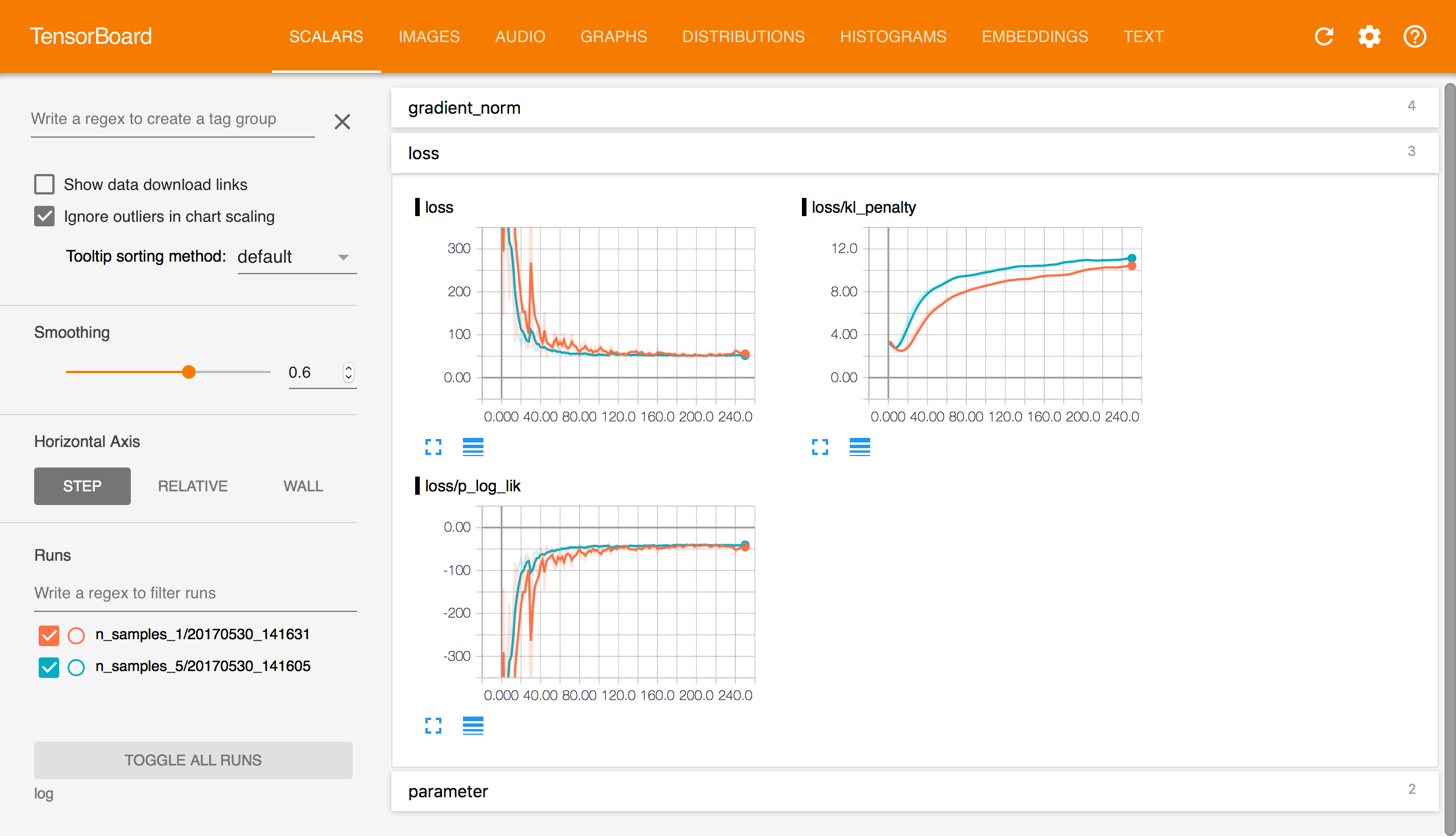
TensorBoard Scalars.

Scalars provides scalar-valued information across iterations of the algorithm, wall time, and relative wall time. In Edward, the tab includes the value of scalar TensorFlow variables (free parameters) in the model or approximating family.

With variational inference, we also include information such as the loss function and its decomposition into individual terms. This particular example shows that n_samples=1 tends to have higher variance than n_samples=5 but still converges to the same solution.

TensorBoard Graphs.

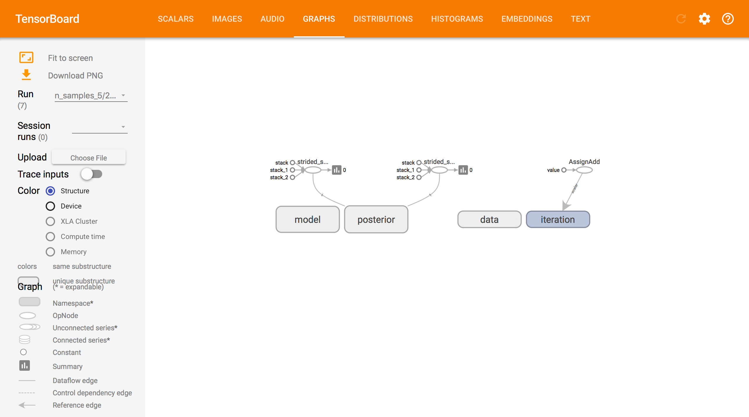
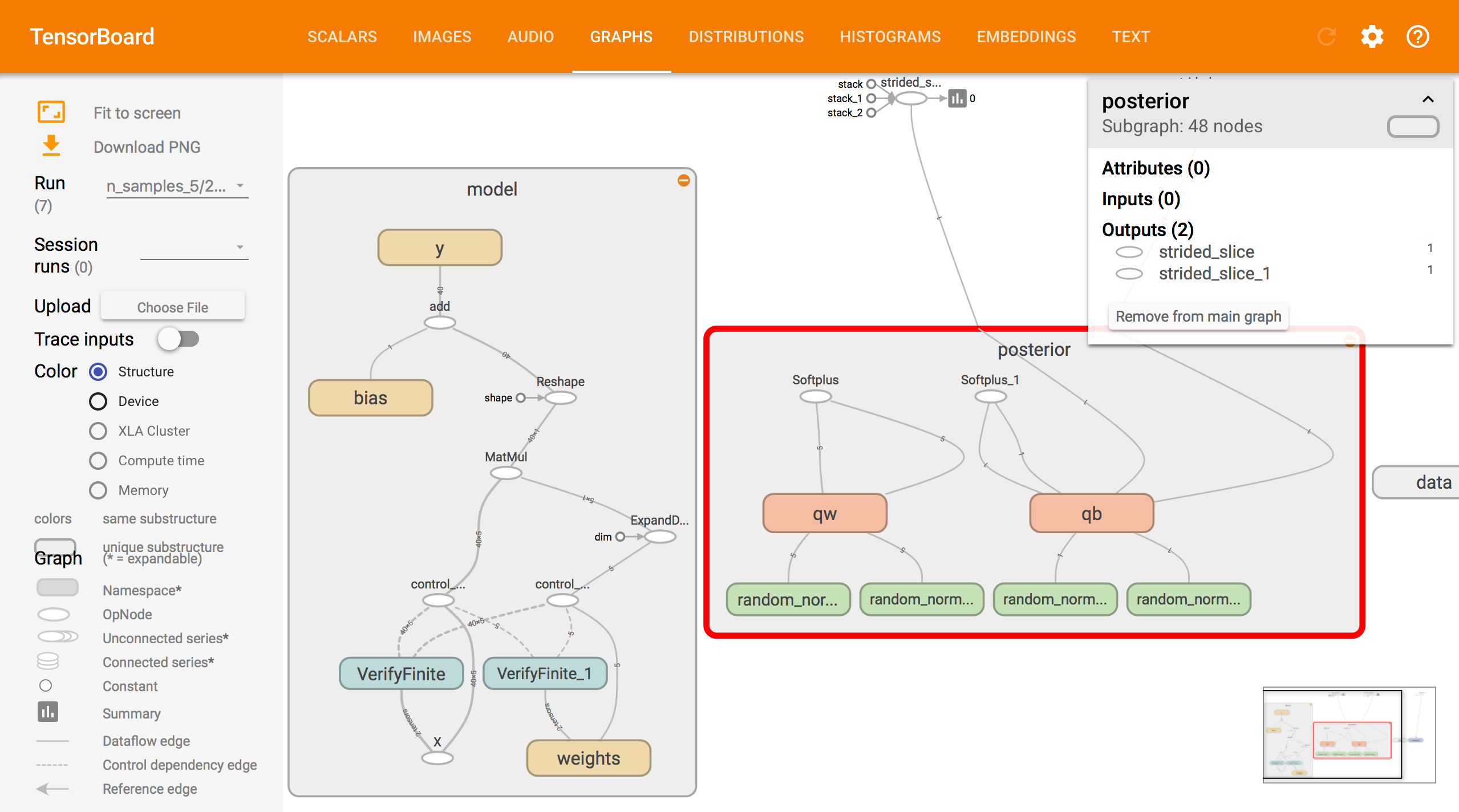
Graphs displays the computational graph underlying the model, approximating family, and inference. Boxes denote tensors grouped under the same name scope. Cleaning up names in the graph makes it easy to better understand and optimize your code.

TensorBoard Distributions.

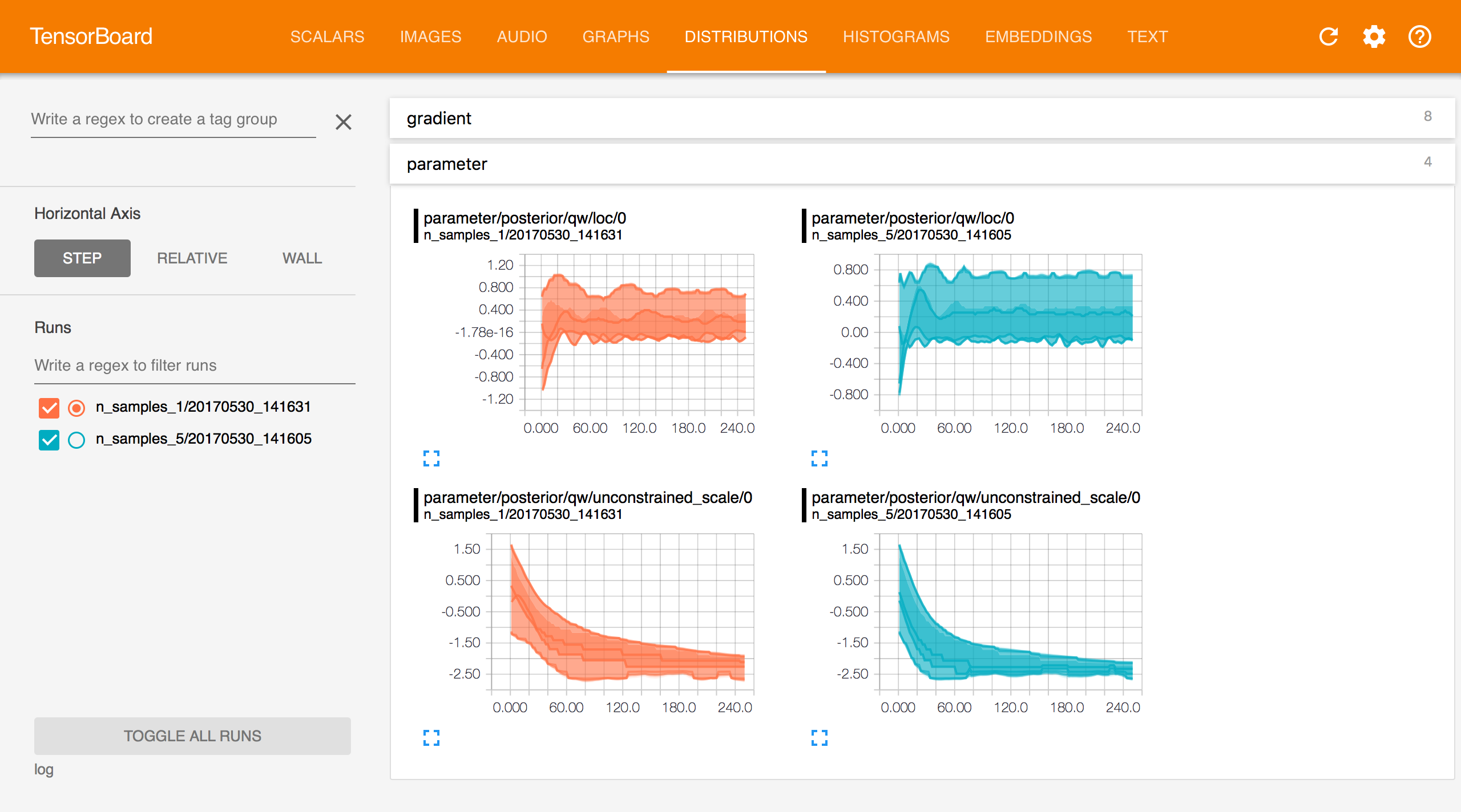
Distributions displays the distribution of each non-scalar TensorFlow variable across iterations. These variables are the free parameters of your model and approximating family.

TensorBoard Histograms.

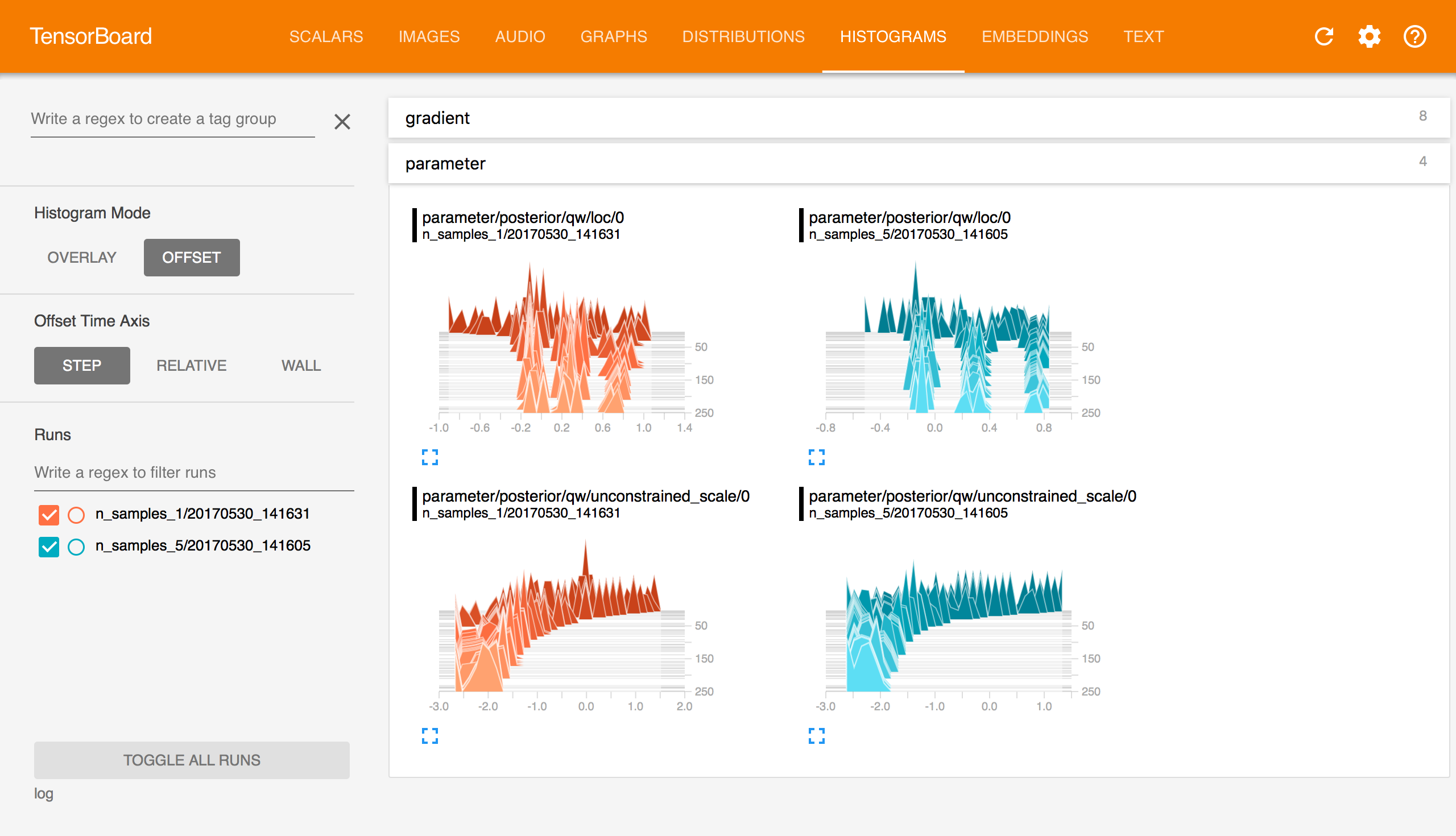
Histograms displays the same information as Distributions but as a 3-D histogram changing aross iteration.

Acknowledgments

We thank Sean Kruzel for writing the initial version of this tutorial.

A TensorFlow tutorial to TensorBoard can be found here.

References

Murphy, K. P. (2012). Machine learning: A probabilistic perspective. MIT Press.