Edward

Getting Started

Getting started with Edward is easy.

Installation

To install the latest stable version, run

pip install edward

To install the latest development version, run

pip install -e "git+https://github.com/blei-lab/edward.git#egg=edward"

See the troubleshooting page for Edward’s dependencies and more details.

Your first Edward program

Probabilistic modeling in Edward uses a simple language of random variables. Here we will show a Bayesian neural network. It is a neural network with a prior distribution on its weights. (This example is abridged; an interactive version with Jupyter notebook is available here.)

First, simulate a toy dataset of 50 observations with a cosine relationship.

import numpy as np

x_train = np.linspace(-3, 3, num=50)
y_train = np.cos(x_train) + np.random.normal(0, 0.1, size=50)
x_train = x_train.astype(np.float32).reshape((50, 1))
y_train = y_train.astype(np.float32).reshape((50, 1))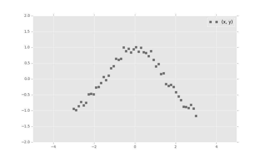

Next, define a two-layer Bayesian neural network. Here, we define the neural network manually with tanh nonlinearities.

import tensorflow as tf
from edward.models import Normal

W_0 = Normal(loc=tf.zeros([1, 2]), scale=tf.ones([1, 2]))
W_1 = Normal(loc=tf.zeros([2, 1]), scale=tf.ones([2, 1]))
b_0 = Normal(loc=tf.zeros(2), scale=tf.ones(2))
b_1 = Normal(loc=tf.zeros(1), scale=tf.ones(1))

x = x_train
y = Normal(loc=tf.matmul(tf.tanh(tf.matmul(x, W_0) + b_0), W_1) + b_1,
           scale=0.1)

Next, make inferences about the model from data. We will use variational inference. Specify a normal approximation over the weights and biases.

qW_0 = Normal(loc=tf.get_variable("qW_0/loc", [1, 2]),
              scale=tf.nn.softplus(tf.get_variable("qW_0/scale", [1, 2])))
qW_1 = Normal(loc=tf.get_variable("qW_1/loc", [2, 1]),
              scale=tf.nn.softplus(tf.get_variable("qW_1/scale", [2, 1])))
qb_0 = Normal(loc=tf.get_variable("qb_0/loc", [2]),
              scale=tf.nn.softplus(tf.get_variable("qb_0/scale", [2])))
qb_1 = Normal(loc=tf.get_variable("qb_1/loc", [1]),
              scale=tf.nn.softplus(tf.get_variable("qb_1/scale", [1])))

Defining tf.get_variable allows the variational factors’ parameters to vary. They are all initialized at 0. The standard deviation parameters are constrained to be greater than zero according to a softplus transformation.

Now, run variational inference with the Kullback-Leibler divergence in order to infer the model’s latent variables given data. We specify 1000 iterations.

import edward as ed

inference = ed.KLqp({W_0: qW_0, b_0: qb_0,
                     W_1: qW_1, b_1: qb_1}, data={y: y_train})
inference.run(n_iter=1000)

Finally, criticize the model fit. Bayesian neural networks define a distribution over neural networks, so we can perform a graphical check. Draw neural networks from the inferred model and visualize how well it fits the data.

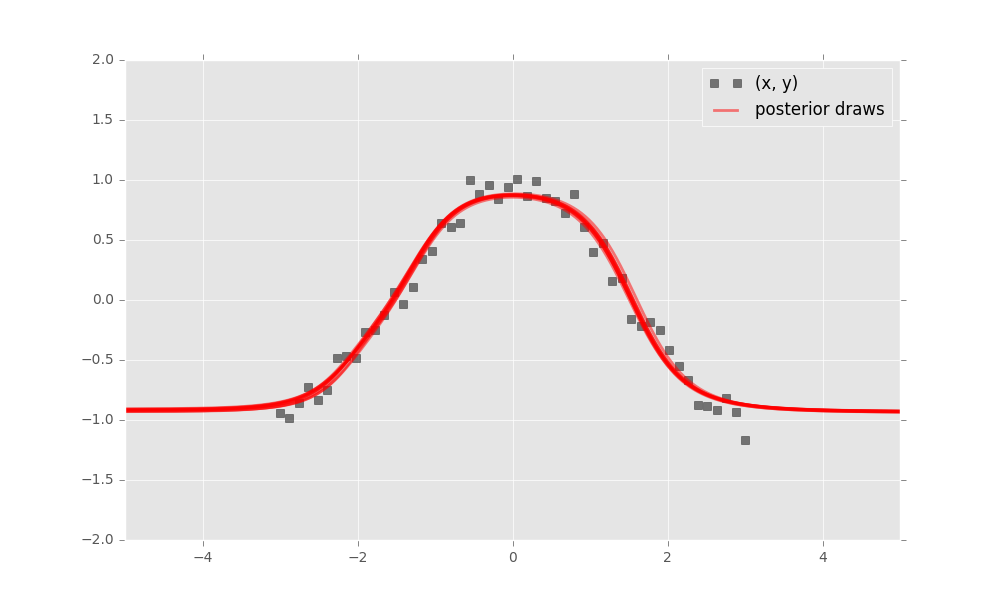
The model has captured the cosine relationship between \(x\) and \(y\) in the observed domain.

To learn more about Edward, delve in!

If you prefer to learn via examples, then check out some tutorials.