Edward

Mixture Density Networks

Mixture density networks (MDN) (Bishop, 1994) are a class of models obtained by combining a conventional neural network with a mixture density model.

We demonstrate with an example in Edward. An interactive version with Jupyter notebook is available here.

Data

We use the same toy data from David Ha’s blog post, where he explains MDNs. It is an inverse problem where for every input \(x_n\) there are multiple outputs \(y_n\).

from sklearn.model_selection import train_test_split

def build_toy_dataset(N):
  y_data = np.random.uniform(-10.5, 10.5, N)
  r_data = np.random.normal(size=N)  # random noise
  x_data = np.sin(0.75 * y_data) * 7.0 + y_data * 0.5 + r_data * 1.0
  x_data = x_data.reshape((N, 1))
  return train_test_split(x_data, y_data, random_state=42)

N = 5000  # number of data points
D = 1  # number of features

X_train, X_test, y_train, y_test = build_toy_dataset(N)
print("Size of features in training data: {}".format(X_train.shape))
print("Size of output in training data: {}".format(y_train.shape))
print("Size of features in test data: {}".format(X_test.shape))
print("Size of output in test data: {}".format(y_test.shape))

sns.regplot(X_train, y_train, fit_reg=False)

## Size of features in training data: (3750, 1)
## Size of output in training data: (3750,)
## Size of features in test data: (1250, 1)
## Size of output in test data: (1250,)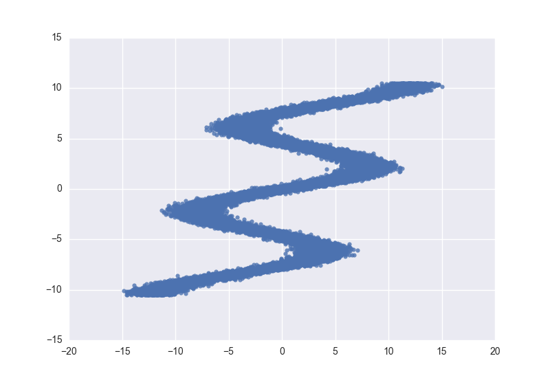

We define TensorFlow placeholders, which will be used to manually feed batches of data during inference. This is one of many ways to train models with data in Edward.

X_ph = tf.placeholder(tf.float32, [None, D])
y_ph = tf.placeholder(tf.float32, [None])

Model

We use a mixture of 20 normal distributions parameterized by a feedforward network. That is, the membership probabilities and per-component mean and standard deviation are given by the output of a feedforward network.

We use tf.layers to construct neural networks. We specify a three-layer network with 15 hidden units for each hidden layer.

from edward.models import Categorical, Mixture, Normal

def neural_network(X):
  """loc, scale, logits = NN(x; theta)"""
  # 2 hidden layers with 15 hidden units
  net = tf.layers.dense(X, 15, activation=tf.nn.relu)
  net = tf.layers.dense(net, 15, activation=tf.nn.relu)
  locs = tf.layers.dense(net, K, activation=None)
  scales = tf.layers.dense(net, K, activation=tf.exp)
  logits = tf.layers.dense(net, K, activation=None)
  return locs, scales, logits

K = 20  # number of mixture components

locs, scales, logits = neural_network(X_ph)
cat = Categorical(logits=logits)
components = [Normal(loc=loc, scale=scale) for loc, scale
              in zip(tf.unstack(tf.transpose(locs)),
                     tf.unstack(tf.transpose(scales)))]
y = Mixture(cat=cat, components=components, value=tf.zeros_like(y_ph))

Note that we use the Mixture random variable. It collapses out the membership assignments for each data point and makes the model differentiable with respect to all its parameters. It takes a Categorical random variable as input—denoting the probability for each cluster assignment—as well as components, which is a list of individual distributions to mix over.

For more background on MDNs, take a look at Christopher Bonnett’s blog post or at Bishop (1994).

Inference

We use MAP estimation, passing in the model and data set. See this extended tutorial about MAP estimation in Edward.

inference = ed.MAP(data={y: y_ph})

Here, we will manually control the inference and how data is passed into it at each step. Initialize the algorithm and the TensorFlow variables.

optimizer = tf.train.AdamOptimizer(5e-3)
inference.initialize(optimizer=optimizer, var_list=tf.trainable_variables())

sess = ed.get_session()
tf.global_variables_initializer().run()

Now we train the MDN by calling inference.update(), passing in the data. The quantity inference.loss is the loss function (negative log-likelihood) at that step of inference. We also report the loss function on test data by calling inference.loss and where we feed test data to the TensorFlow placeholders instead of training data. We keep track of the losses under train_loss and test_loss.

n_epoch = 1000
train_loss = np.zeros(n_epoch)
test_loss = np.zeros(n_epoch)
for i in range(n_epoch):
  info_dict = inference.update(feed_dict={X_ph: X_train, y_ph: y_train})
  train_loss[i] = info_dict['loss']
  test_loss[i] = sess.run(inference.loss, feed_dict={X_ph: X_test, y_ph: y_test})
  inference.print_progress(info_dict)

Note a common failure mode when training MDNs is that an individual mixture distribution collapses to a point. This forces the standard deviation of the normal to be close to 0 and produces NaN values. We can prevent this by thresholding the standard deviation if desired.

After training for a number of iterations, we get out the predictions we are interested in from the model: the predicted mixture weights, cluster means, and cluster standard deviations.

To do this, we fetch their values from session, feeding test data X_test to the placeholder X_ph.

pred_weights, pred_means, pred_std = sess.run(
    [tf.nn.softmax(logits), locs, scales], feed_dict={X_ph: X_test})

Let’s plot the log-likelihood of the training and test data as functions of the training epoch. The quantity inference.loss is the total log-likelihood, not the loss per data point. Below we plot the per-data point log-likelihood by dividing by the size of the train and test data respectively.

fig, axes = plt.subplots(nrows=1, ncols=1, figsize=(16, 3.5))
plt.plot(np.arange(n_epoch), -test_loss / len(X_test), label='Test')
plt.plot(np.arange(n_epoch), -train_loss / len(X_train), label='Train')
plt.legend(fontsize=20)
plt.xlabel('Epoch', fontsize=15)
plt.ylabel('Log-likelihood', fontsize=15)
plt.show()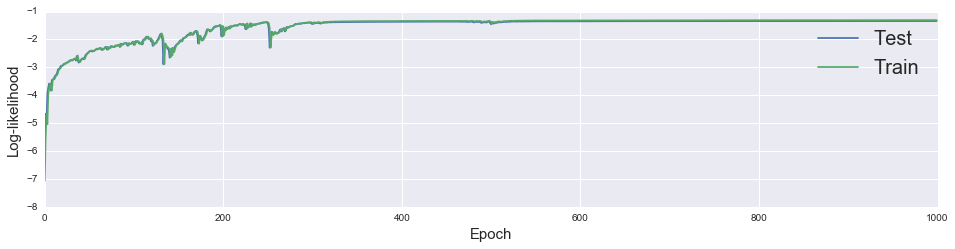

We see that it converges after roughly 400 iterations.

Criticism

Let’s look at how individual examples perform. Note that as this is an inverse problem we can’t get the answer correct, but we can hope that the truth lies in area where the model has high probability.

In this plot the truth is the vertical grey line while the blue line is the prediction of the mixture density network. As you can see, we didn’t do too bad.

obj = [0, 4, 6]
fig, axes = plt.subplots(nrows=3, ncols=1, figsize=(16, 6))

plot_normal_mix(pred_weights[obj][0], pred_means[obj][0], pred_std[obj][0], axes[0], comp=False)
axes[0].axvline(x=y_test[obj][0], color='black', alpha=0.5)

plot_normal_mix(pred_weights[obj][2], pred_means[obj][2], pred_std[obj][2], axes[1], comp=False)
axes[1].axvline(x=y_test[obj][2], color='black', alpha=0.5)

plot_normal_mix(pred_weights[obj][1], pred_means[obj][1], pred_std[obj][1], axes[2], comp=False)
axes[2].axvline(x=y_test[obj][1], color='black', alpha=0.5)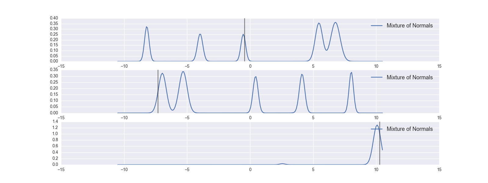

We can check the ensemble by drawing samples of the prediction and plotting the density of those. The MDN has learned what we’d like it to learn.

a = sample_from_mixture(X_test, pred_weights, pred_means, pred_std, amount=len(X_test))
sns.jointplot(a[:,0], a[:,1], kind="hex", color="#4CB391", ylim=(-10,10), xlim=(-14,14))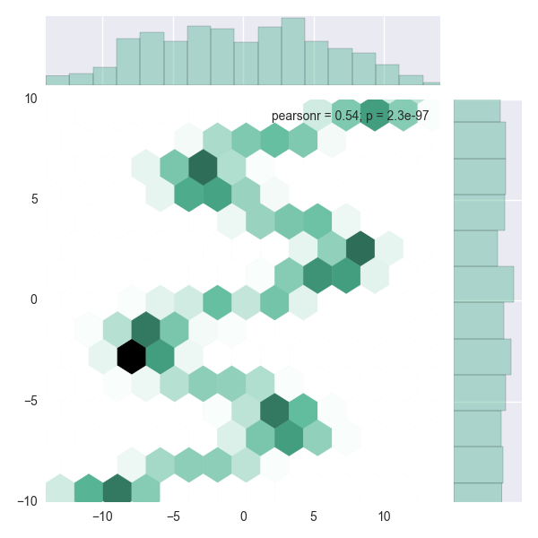

Acknowledgments

We thank Christopher Bonnett for writing the initial version of this tutorial. More generally, we thank Chris for pushing forward momentum to have Edward tutorials be accessible and easy-to-learn.

References

Bishop, C. M. (1994). Mixture density networks.