Edward

Linear Mixed Effects Models

With linear mixed effects models, we wish to model a linear relationship for data points with inputs of varying type, categorized into subgroups, and associated to a real-valued output.

We demonstrate with an example in Edward. An interactive version with Jupyter notebook is available here.

Data

We use the InstEval data set from the popular lme4 R package (Bates, Mächler, Bolker, & Walker, 2015). It is a data set of instructor evaluation ratings, where the inputs (covariates) include categories such as students and departments, and our response variable of interest is the instructor evaluation rating.

import pandas as pd
from observations import insteval

data, metadata = insteval("~/data")
data = pd.DataFrame(data, columns=metadata['columns'])

# s - students - 1:2972
# d - instructors - codes that need to be remapped
# dept also needs to be remapped
data['s'] = data['s'] - 1
data['dcodes'] = data['d'].astype('category').cat.codes
data['deptcodes'] = data['dept'].astype('category').cat.codes
data['y'] = data['y'].values.astype(float)

train = data.sample(frac=0.8)
test = data.drop(train.index)

The data set denotes:

• students as s
• instructors as d
• departments as dept
• service as service

s_train = train['s'].values
d_train = train['dcodes'].values
dept_train = train['deptcodes'].values
y_train = train['y'].values
service_train = train['service'].values
n_obs_train = train.shape[0]

s_test = test['s'].values
d_test = test['dcodes'].values
dept_test = test['deptcodes'].values
y_test = test['y'].values
service_test = test['service'].values
n_obs_test = test.shape[0]

n_s = max(s_train) + 1  # number of students
n_d = max(d_train) + 1  # number of instructors
n_dept = max(dept_train) + 1  # number of departments
n_obs = train.shape[0]  # number of observations

print("Number of students: {}".format(n_s))
print("Number of instructors: {}".format(n_d))
print("Number of departments: {}".format(n_dept))
print("Number of observations: {}".format(n_obs))

Number of students: 2972
Number of instructors: 1128
Number of departments: 14
Number of observations: 58737

Model

With linear regression, one makes an independence assumption where each data point regresses with a constant slope among each other. In our setting, the observations come from groups which may have varying slopes and intercepts. Thus we’d like to build a model that can capture this behavior (Gelman & Hill, 2006).

For examples of this phenomena:

• The observations from a single student are not independent of each other. Rather, some students may systematically give low (or high) lecture ratings.
• The observations from a single teacher are not independent of each other. We expect good teachers to get generally good ratings and bad teachers to get generally bad ratings.
• The observations from a single department are not independent of each other. One department may generally have dry material and thus be rated lower than others.

Typical linear regression takes the form \[\mathbf{y} = \mathbf{X}\beta + \epsilon,\] where \(\mathbf{X}\) corresponds to fixed effects with coefficients \(\beta\) and \(\epsilon\) corresponds to random noise, \(\epsilon\sim\mathcal{N}(\mathbf{0}, \mathbf{I})\).

In a linear mixed effects model, we add an additional term \(\mathbf{Z}\eta\), where \(\mathbf{Z}\) corresponds to random effects with coefficients \(\eta\). The model takes the form \[\begin{aligned} \eta &\sim \mathcal{N}(\mathbf{0}, \sigma^2 \mathbf{I}), \\ \mathbf{y} &= \mathbf{X}\beta + \mathbf{Z}\eta + \epsilon.\end{aligned}\] Given data, the goal is to infer \(\beta\), \(\eta\), and \(\sigma^2\), where \(\beta\) are model parameters (“fixed effects”), \(\eta\) are latent variables (“random effects”), and \(\sigma^2\) is a variance component parameter.

Because the random effects have mean 0, the data’s mean is captured by \(\mathbf{X}\beta\). The random effects component \(\mathbf{Z}\eta\) captures variations in the data (e.g. Instructor #54 is rated 1.4 points higher than the mean).

A natural question is the difference between fixed and random effects. A fixed effect is an effect that is constant for a given population. A random effect is an effect that varies for a given population (i.e., it may be constant within subpopulations but varies within the overall population). We illustrate below in our example:

• Select service as the fixed effect. It is a binary covariate corresponding to whether the lecture belongs to the lecturer’s main department. No matter how much additional data we collect, it can only take on the values in \(0\) and \(1\).
• Select the categorical values of students, teachers, and departments as the random effects. Given more observations from the population of instructor evaluation ratings, we may be looking at new students, teachers, or departments.

In the syntax of R’s lme4 package (Bates et al., 2015), the model can be summarized as

y ~ 1 + (1|students) + (1|instructor) + (1|dept) + service

where 1 denotes an intercept term, (1|x) denotes a random effect for x, and x denotes a fixed effect.

# Set up placeholders for the data inputs.
s_ph = tf.placeholder(tf.int32, [None])
d_ph = tf.placeholder(tf.int32, [None])
dept_ph = tf.placeholder(tf.int32, [None])
service_ph = tf.placeholder(tf.float32, [None])

# Set up fixed effects.
mu = tf.get_variable("mu", [])
service = tf.get_variable("service", [])

sigma_s = tf.sqrt(tf.exp(tf.get_variable("sigma_s", [])))
sigma_d = tf.sqrt(tf.exp(tf.get_variable("sigma_d", [])))
sigma_dept = tf.sqrt(tf.exp(tf.get_variable("sigma_dept", [])))

# Set up random effects.
eta_s = Normal(loc=tf.zeros(n_s), scale=sigma_s * tf.ones(n_s))
eta_d = Normal(loc=tf.zeros(n_d), scale=sigma_d * tf.ones(n_d))
eta_dept = Normal(loc=tf.zeros(n_dept), scale=sigma_dept * tf.ones(n_dept))

yhat = (tf.gather(eta_s, s_ph) +
        tf.gather(eta_d, d_ph) +
        tf.gather(eta_dept, dept_ph) +
        mu + service * service_ph)
y = Normal(loc=yhat, scale=tf.ones(n_obs))

Inference

Given data, we aim to infer the model’s fixed and random effects. In this analysis, we use variational inference with the \(\text{KL}(q\|p)\) divergence measure. We specify fully factorized normal approximations for the random effects and pass in all training data for inference. Under the algorithm, the fixed effects will be estimated under a variational EM scheme.

q_eta_s = Normal(
    loc=tf.get_variable("q_eta_s/loc", [n_s]),
    scale=tf.nn.softplus(tf.get_variable("q_eta_s/scale", [n_s])))
q_eta_d = Normal(
    loc=tf.get_variable("q_eta_d/loc", [n_d]),
    scale=tf.nn.softplus(tf.get_variable("q_eta_d/scale", [n_d])))
q_eta_dept = Normal(
    loc=tf.get_variable("q_eta_dept/loc", [n_dept]),
    scale=tf.nn.softplus(tf.get_variable("q_eta_dept/scale", [n_dept])))

latent_vars = {
    eta_s: q_eta_s,
    eta_d: q_eta_d,
    eta_dept: q_eta_dept}
data = {
    y: y_train,
    s_ph: s_train,
    d_ph: d_train,
    dept_ph: dept_train,
    service_ph: service_train}
inference = ed.KLqp(latent_vars, data)

One way to critique the fitted model is a residual plot, i.e., a plot of the difference between the predicted value and the observed value for each data point. Below we manually run inference, initializing the algorithm and performing individual updates within a loop. We form residual plots as the algorithm progresses. This helps us examine how the algorithm proceeds to infer the random and fixed effects from data.

To form residuals, we first make predictions on test data. We do this by copying yhat defined in the model and replacing its dependence on random effects with their inferred means. During the algorithm, we evaluate the predictions, feeding in test inputs.

We have also fit the same model (y   service + (1|dept) + (1|s) + (1|d), fit on the entire InstEval dataset, specifically) in lme4. We have saved the random effect estimates and will compare them to our learned parameters.

yhat_test = ed.copy(yhat, {
    eta_s: q_eta_s.mean(),
    eta_d: q_eta_d.mean(),
    eta_dept: q_eta_dept.mean()})

We now write the main loop.

inference.initialize(n_print=20, n_iter=100)
tf.global_variables_initializer().run()

for _ in range(inference.n_iter):
  # Update and print progress of algorithm.
  info_dict = inference.update()
  inference.print_progress(info_dict)

  t = info_dict['t']
  if t == 1 or t % inference.n_print == 0:
    # Make predictions on test data.
    yhat_vals = yhat_test.eval(feed_dict={
        s_ph: s_test,
        d_ph: d_test,
        dept_ph: dept_test,
        service_ph: service_test})

    # Form residual plot.
    plt.title("Residuals for Predicted Ratings on Test Set")
    plt.xlim(-4, 4)
    plt.ylim(0, 800)
    plt.hist(yhat_vals - y_test, 75)
    plt.show()

Criticism

Above, we described a method for diagnosing the fit of the model via residual plots. Below we show the residuals for the model post-convergence. (For intermediate residual plots, check the Jupyter notebook.)

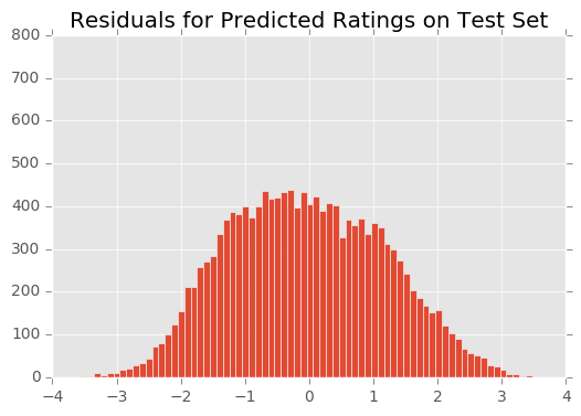
The residuals appear normally distributed with mean 0. The residuals appear normally distributed with mean 0. This is a good sanity check for the model.

We can also compare our learned parameters to those estimated by R’s ‘lme4‘.

student_effects_lme4 = pd.read_csv('data/insteval_student_ranefs_r.csv')
instructor_effects_lme4 = pd.read_csv('data/insteval_instructor_ranefs_r.csv')
dept_effects_lme4 = pd.read_csv('data/insteval_dept_ranefs_r.csv')

student_effects_edward = q_eta_s.mean().eval()
instructor_effects_edward = q_eta_d.mean().eval()
dept_effects_edward = q_eta_dept.mean().eval()

plt.title("Student Effects Comparison")
plt.xlim(-1, 1)
plt.ylim(-1, 1)
plt.xlabel("Student Effects from lme4")
plt.ylabel("Student Effects from edward")
plt.scatter(student_effects_lme4["(Intercept)"],
            student_effects_edward,
            alpha=0.25)
plt.show()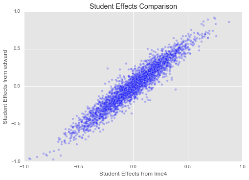

plt.title("Instructor Effects Comparison")
plt.xlim(-1.5, 1.5)
plt.ylim(-1.5, 1.5)
plt.xlabel("Instructor Effects from lme4")
plt.ylabel("Instructor Effects from edward")
plt.scatter(instructor_effects_lme4["(Intercept)"],
            instructor_effects_edward,
            alpha=0.25)
plt.show()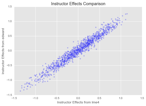

Great! Our estimates for both student and instructor effects seem to match those from ‘lme4‘ closely. We have set up a slightly different model here (for example, our overall mean is regularized, as are our variances for student, department, and instructor effects, which is not true of ‘lme4‘s model), and we have a different inference method, so we should not expect to find exactly the same parameters as ‘lme4‘. But it is reassuring that they match up closely!

#  Add in the intercept from R and edward
dept_effects_and_intercept_lme4 = 3.28259 + dept_effects_lme4["(Intercept)"]
dept_effects_and_intercept_edward = mu.eval() + dept_effects_edward

plt.title("Departmental Effects Comparison")
plt.xlim(3.0, 3.5)
plt.ylim(3.0, 3.5)
plt.xlabel("Department Effects from lme4")
plt.ylabel("Department Effects from edward")
plt.scatter(dept_effects_and_intercept_lme4,
            dept_effects_and_intercept_edward,
            s=0.01 * train.dept.value_counts())
plt.show()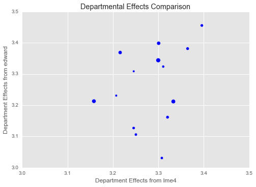

Our department effects do not match up nearly as well with those from ‘lme4‘. There are likely several reasons for this:

• We regularize the overall mean, while ‘lme4‘ doesn’t. This causes the Edward model to put some of the intercept into the department effects, which are allowed to vary more widely since we learn a variance
• We are using 80 estimate uses the whole ‘InstEval‘ data set
• The department effects are the weakest in the model and difficult to estimate.

Acknowledgments

We thank Mayank Agrawal for writing the initial version of this tutorial.

References

Bates, D., Mächler, M., Bolker, B., & Walker, S. (2015). Fitting Linear Mixed-Effects Models Using lme4. Journal of Statistical Software, 67(1), 1–48.
Gelman, A., & Hill, J. L. (2006). Data analysis using regression and multilevel/hierarchical models. Cambridge University Press.