Edward

Generative Adversarial Networks

Generative adversarial networks (GANs) are a powerful approach for probabilistic modeling (Goodfellow, 2016; I. Goodfellow et al., 2014). They posit a deep generative model and they enable fast and accurate inferences.

We demonstrate with an example in Edward. An interactive version with Jupyter notebook is available here.

M = 128  # batch size during training
d = 100  # latent dimension

data_dir = "/tmp/data"
out_dir = "/tmp/out"

Data

We use training data from MNIST, which consists of 55,000 \(28\times 28\) pixel images (LeCun, Bottou, Bengio, & Haffner, 1998). Each image is represented as a flattened vector of 784 elements, and each element is a pixel intensity between 0 and 1.

The goal is to build and infer a model that can generate high quality images of handwritten digits.

During training we will feed batches of MNIST digits. We instantiate a TensorFlow placeholder with a fixed batch size of \(M\) images.

We also define a helper function to select the next batch of data points from the full set of examples. It keeps track of the current batch index and returns the next batch using the function next(). We will generate batches from x_train_generator during inference.

from observations import mnist

def generator(array, batch_size):
  """Generate batch with respect to array's first axis."""
  start = 0  # pointer to where we are in iteration
  while True:
    stop = start + batch_size
    diff = stop - array.shape[0]
    if diff <= 0:
      batch = array[start:stop]
      start += batch_size
    else:
      batch = np.concatenate((array[start:], array[:diff]))
      start = diff
    batch = batch.astype(np.float32) / 255.0  # normalize pixel intensities
    batch = np.random.binomial(1, batch)  # binarize images
    yield batch

(x_train, _), (x_test, _) = mnist(data_dir)
x_train_generator = generator(x_train, M)
x_ph = tf.placeholder(tf.float32, [M, 784])

Model

GANs posit generative models using an implicit mechanism. Given some random noise, the data is assumed to be generated by a deterministic function of that noise.

Formally, the generative process is \[\begin{aligned} \mathbf{\epsilon} &\sim p(\mathbf{\epsilon}), \\ \mathbf{x} &= G(\mathbf{\epsilon}; \theta),\end{aligned}\] where \(G(\cdot; \theta)\) is a neural network that takes the samples \(\mathbf{\epsilon}\) as input. The distribution \(p(\mathbf{\epsilon})\) is interpreted as random noise injected to produce stochasticity in a physical system; it is typically a fixed uniform or normal distribution with some latent dimensionality.

In Edward, we build the model as follows, using tf.layers to specify the neural network. It defines a 2-layer fully connected neural network and outputs a vector of length \(28\times28\) with values in \([0,1]\).

from edward.models import Uniform

def generative_network(eps):
  net = tf.layers.dense(eps, 128, activation=tf.nn.relu)
  net = tf.layers.dense(net, 784, activation=tf.sigmoid)
  return net

with tf.variable_scope("Gen"):
  eps = Uniform(tf.zeros([M, d]) - 1.0, tf.ones([M, d]))
  x = generative_network(eps)

We aim to estimate parameters of the generative network such that the model best captures the data. (Note in GANs, we are interested only in parameter estimation and not inference about any latent variables.)

Unfortunately, probability models described above do not admit a tractable likelihood. This poses a problem for most inference algorithms, as they usually require taking the model’s density. Thus we are motivated to use “likelihood-free” algorithms (Marin, Pudlo, Robert, & Ryder, 2012), a class of methods which assume one can only sample from the model.

Inference

A key idea in likelihood-free methods is to learn by comparison (e.g., Rubin (1984; Gretton, Borgwardt, Rasch, Schölkopf, & Smola, 2012)): by analyzing the discrepancy between samples from the model and samples from the true data distribution, we have information on where the model can be improved in order to generate better samples.

In GANs, a neural network \(D(\cdot;\phi)\) makes this comparison, known as the discriminator. \(D(\cdot;\phi)\) takes data \(\mathbf{x}\) as input (either generations from the model or data points from the data set), and it calculates the probability that \(\mathbf{x}\) came from the true data.

In Edward, we use the following discriminative network. It is simply a feedforward network with one ReLU hidden layer. It returns the probability in the logit (unconstrained) scale.

def discriminative_network(x):
  """Outputs probability in logits."""
  net = tf.layers.dense(x, 128, activation=tf.nn.relu)
  net = tf.layers.dense(net, 1, activation=None)
  return net

Let \(p^*(\mathbf{x})\) represent the true data distribution. The optimization problem used in GANs is

\[\min_\theta \max_\phi~ \mathbb{E}_{p^*(\mathbf{x})} [ \log D(\mathbf{x}; \phi) ] + \mathbb{E}_{p(\mathbf{x}; \theta)} [ \log (1 - D(\mathbf{x}; \phi)) ].\]

This optimization problem is bilevel: it requires a minima solution with respect to generative parameters and a maxima solution with respect to discriminative parameters. In practice, the algorithm proceeds by iterating gradient updates on each. An additional heuristic also modifies the objective function for the generative model in order to avoid saturation of gradients (I. J. Goodfellow, 2014).

Many sources of intuition exist behind GAN-style training. One, which is the original motivation, is based on idea that the two neural networks are playing a game. The discriminator tries to best distinguish samples away from the generator. The generator tries to produce samples that are indistinguishable by the discriminator. The goal of training is to reach a Nash equilibrium.

Another source is the idea of casting unsupervised learning as supervised learning (Gutmann & Hyvärinen, 2010; Gutmann, Dutta, Kaski, & Corander, 2014). This allows one to leverage the power of classification—a problem that in recent years is (relatively speaking) very easy.

A third comes from classical statistics, where the discriminator is interpreted as a proxy of the density ratio between the true data distribution and the model (Mohamed & Lakshminarayanan, 2016; Sugiyama, Suzuki, & Kanamori, 2012). By augmenting an original problem that may require the model’s density with a discriminator (such as maximum likelihood), one can recover the original problem when the discriminator is optimal. Furthermore, this approximation is very fast, and it justifies GANs from the perspective of approximate inference.

In Edward, the GAN algorithm (GANInference) simply takes the implicit density model on x as input, binded to its realizations x_ph. In addition, a parameterized function discriminator is provided to distinguish their samples.

inference = ed.GANInference(
    data={x: x_ph}, discriminator=discriminative_network)

We’ll use ADAM as optimizers for both the generator and discriminator. We’ll run the algorithm for 15,000 iterations and print progress every 1,000 iterations.

optimizer = tf.train.AdamOptimizer()
optimizer_d = tf.train.AdamOptimizer()

inference.initialize(
    optimizer=optimizer, optimizer_d=optimizer_d,
    n_iter=15000, n_print=1000)

We now form the main loop which trains the GAN. At each iteration, it takes a minibatch and updates the parameters according to the algorithm. At every 1000 iterations, it will print progress and also saves a figure of generated samples from the model.

sess = ed.get_session()
tf.global_variables_initializer().run()

idx = np.random.randint(M, size=16)
i = 0
for t in range(inference.n_iter):
  if t % inference.n_print == 0:
    samples = sess.run(x)
    samples = samples[idx, ]

    fig = plot(samples)
    plt.savefig(os.path.join(out_dir, '{}.png').format(
        str(i).zfill(3)), bbox_inches='tight')
    plt.close(fig)
    i += 1

  x_batch = next(x_train_generator)
  info_dict = inference.update(feed_dict={x_ph: x_batch})
  inference.print_progress(info_dict)

Examining convergence of the GAN objective can be meaningless in practice. The algorithm is usually run until some other criterion is satisfied, such as if the samples look visually okay, or if the GAN can capture meaningful parts of the data.

Criticism

Evaluation of GANs remains an open problem—both in criticizing their fit to data and in assessing convergence. Recent advances have considered alternative objectives and heuristics to stabilize training (see also Soumith Chintala’s GAN hacks repo).

As one approach to criticize the model, we simply look at generated images during training. Below we show generations after 14,000 iterations (that is, 14,000 gradient updates of both the generator and the discriminator).

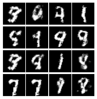
The images are meaningful albeit a little blurry. Suggestions for further improvements would be to tune the hyperparameters in the optimization, to improve the capacity of the discriminative and generative networks, and to leverage more prior information (such as convolutional architectures).

References

Goodfellow, I. (2016). NIPS 2016 Tutorial: Generative Adversarial Networks. arXiv Preprint arXiv:1701.00160.
Goodfellow, I. J. (2014). On distinguishability criteria for estimating generative models. In ICLR workshop.
Goodfellow, I., Pouget-Abadie, J., Mirza, M., Xu, B., Warde-Farley, D., Ozair, S., … Bengio, Y. (2014). Generative adversarial nets. In Neural information processing systems.
Gretton, A., Borgwardt, K. M., Rasch, M. J., Schölkopf, B., & Smola, A. (2012). A kernel two-sample test. The Journal of Machine Learning Research, 13, 723–773.
Gutmann, M., & Hyvärinen, A. (2010). Noise-contrastive estimation: A new estimation principle for unnormalized statistical models. In Artificial intelligence and statistics.
Gutmann, M. U., Dutta, R., Kaski, S., & Corander, J. (2014). Statistical Inference of Intractable Generative Models via Classification. arXiv Preprint arXiv:1407.4981.
LeCun, Y., Bottou, L., Bengio, Y., & Haffner, P. (1998). Gradient-based learning applied to document recognition. Proceedings of the IEEE, 86(11), 2278–2324.
Marin, J.-M., Pudlo, P., Robert, C. P., & Ryder, R. J. (2012). Approximate Bayesian computational methods. Statistics and Computing, 22(6), 1167–1180.
Mohamed, S., & Lakshminarayanan, B. (2016). Learning in Implicit Generative Models. arXiv Preprint arXiv:1610.03483.
Rubin, D. B. (1984). Bayesianly justifiable and relevant frequency calculations for the applied statistician. The Annals of Statistics, 12(4), 1151–1172.
Sugiyama, M., Suzuki, T., & Kanamori, T. (2012). Density-ratio matching under the Bregman divergence: a unified framework of density-ratio estimation. Annals of the Institute of Statistical ….