Edward

Probabilistic PCA

Probabilistic principal components analysis (PCA) is a dimensionality reduction technique that analyzes data via a lower dimensional latent space (Tipping & Bishop, 1999). It is often used when there are missing values in the data or for multidimensional scaling.

We demonstrate with an example in Edward. An interactive version with Jupyter notebook is available here.

Data

We use simulated data. We’ll talk about the individual variables and what they stand for in the next section. For this example, each data point is 2-dimensional, \(\mathbf{x}_n\in\mathbb{R}^2\).

def build_toy_dataset(N, D, K, sigma=1):
  x_train = np.zeros((D, N))
  w = np.random.normal(0.0, 2.0, size=(D, K))
  z = np.random.normal(0.0, 1.0, size=(K, N))
  mean = np.dot(w, z)
  for d in range(D):
    for n in range(N):
      x_train[d, n] = np.random.normal(mean[d, n], sigma)

  print("True principal axes:")
  print(w)
  return x_train

N = 5000  # number of data points
D = 2  # data dimensionality
K = 1  # latent dimensionality

x_train = build_toy_dataset(N, D, K)

## True principal axes:
## [[ 0.25947927]
##  [ 1.80472372]]

We visualize the data set.

plt.scatter(x_train[0, :], x_train[1, :], color='blue', alpha=0.1)
plt.axis([-10, 10, -10, 10])
plt.title("Simulated data set")
plt.show()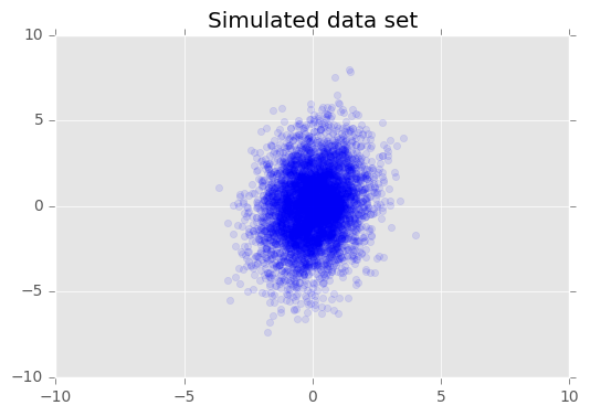

Model

Consider a data set \(\mathbf{X} = \{\mathbf{x}_n\}\) of \(N\) data points, where each data point is \(D\)-dimensional, \(\mathbf{x}_n \in \mathbb{R}^D\). We aim to represent each \(\mathbf{x}_n\) under a latent variable \(\mathbf{z}_n \in \mathbb{R}^K\) with lower dimension, \(K < D\). The set of principal axes \(\mathbf{W}\) relates the latent variables to the data.

Specifically, we assume that each latent variable is normally distributed, \[\mathbf{z}_n \sim N(\mathbf{0}, \mathbf{I}).\] The corresponding data point is generated via a projection, \[\mathbf{x}_n \mid \mathbf{z}_n \sim N(\mathbf{W}\mathbf{z}_n, \sigma^2\mathbf{I}),\] where the matrix \(\mathbf{W}\in\mathbb{R}^{D\times K}\) are known as the principal axes. In probabilistic PCA, we are typically interested in estimating the principal axes \(\mathbf{W}\) and the noise term \(\sigma^2\).

Probabilistic PCA generalizes classical PCA. Marginalizing out the the latent variable, the distribution of each data point is \[\mathbf{x}_n \sim N(\mathbf{0}, \mathbf{W}\mathbf{W}^Y + \sigma^2\mathbf{I}).\] Classical PCA is the specific case of probabilistic PCA when the covariance of the noise becomes infinitesimally small, \(\sigma^2 \to 0\).

We set up our model below. In our analysis, we fix \(\sigma=2.0\), and instead of point estimating \(\mathbf{W}\) as a model parameter, we place a prior over it in order to infer a distribution over principal axes.

from edward.models import Normal

w = Normal(loc=tf.zeros([D, K]), scale=2.0 * tf.ones([D, K]))
z = Normal(loc=tf.zeros([N, K]), scale=tf.ones([N, K]))
x = Normal(loc=tf.matmul(w, z, transpose_b=True), scale=tf.ones([D, N]))

Inference

The posterior distribution over the principal axes \(\mathbf{W}\) cannot be analytically determined. Below, we set up our inference variables and then run a chosen algorithm to infer \(\mathbf{W}\). Below we use variational inference to minimize the \(\text{KL}(q\|p)\) divergence measure.

qw = Normal(loc=tf.get_variable("qw/loc", [D, K]),
            scale=tf.nn.softplus(tf.get_variable("qw/scale", [D, K])))
qz = Normal(loc=tf.get_variable("qz/loc", [N, K]),
            scale=tf.nn.softplus(tf.get_variable("qz/scale", [N, K])))

inference = ed.KLqp({w: qw, z: qz}, data={x: x_train})
inference.run(n_iter=500, n_print=100, n_samples=10)

Criticism

To check our inferences, we first inspect the model’s learned principal axes.

sess = ed.get_session()
print("Inferred principal axes:")
print(sess.run(qw.mean()))

## Inferred principal axes:
## [[-0.24093632]
##  [-1.76468039]]

The model has recovered the true principal axes up to finite data and also up to identifiability (there’s a symmetry in the parameterization).

Another way to criticize the model is to visualize the observed data against data generated from our fitted model.

x_post = ed.copy(x, {w: qw, z: qz})
x_gen = sess.run(x_post)

plt.scatter(x_gen[0, :], x_gen[1, :], color='red', alpha=0.1)
plt.axis([-10, 10, -10, 10])
plt.title("Data generated from model")
plt.show()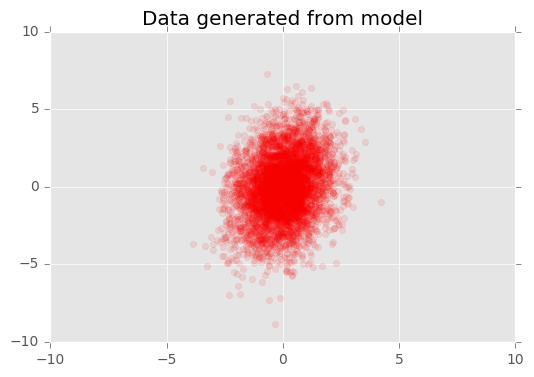

The generated data looks close to the true data.

Acknowledgments

We thank Mayank Agrawal for writing the initial version of this tutorial.

References

Tipping, M. E., & Bishop, C. M. (1999). Probabilistic principal component analysis. Journal of the Royal Statistical Society: Series B (Statistical Methodology), 61(3), 611–622.