Edward

Automated Transformations

Automated transformations provide convenient handling of constrained continuous variables during inference by transforming them to an unconstrained space. Automated transformations are crucial for expanding the scope of algorithm classes such as gradient-based Monte Carlo and variational inference with reparameterization gradients.

A Jupyter notebook version of this tutorial is available here.

The Transform Primitive

Automated transformations in Edward are enabled through the key primitive ed.transform. It takes as input a (possibly constrained) continuous random variable \(\mathbf{x}\), defaults to a choice of transformation \(T\), and returns a TransformedDistribution \(\mathbf{y}=T(\mathbf{x})\) with unconstrained support. An optional argument allows you to manually specify the transformation.

The returned random variable \(\mathbf{y}\)’s density is the original random variable \(\mathbf{x}\)’s density adjusted by the determinant of the Jacobian of the inverse transformation (Casella & Berger, 2002),

\[p(\mathbf{y}) = p(\mathbf{x})~|\mathrm{det}~J_{T^{-1}}(\mathbf{y}) |.\]

Intuitively, the Jacobian describes how a transformation warps unit volumes across spaces. This matters for transformations of random variables, since probability density functions must always integrate to one.

Automated Transformations in Inference

To use automated transformations during inference, set the flag argument auto_transform=True in inference.initialize (or the all-encompassing method inference.run):

inference.initialize(auto_transform=True)

By default, the flag is already set to True. With this flag, any key-value pair passed into inference’s latent_vars with unequal support is transformed to the unconstrained space; no transformation is applied if already unconstrained. The algorithm is then run under inference.latent_vars, which explicitly stores the transformed latent variables and forgets the constrained ones.

We illustrate automated transformations in a few inference examples. Imagine that the target distribution is a Gamma distribution.

from edward.models import Gamma

x = Gamma(1.0, 2.0)

This example is only used for illustration, but note this context of inference with latent variables of non-negative support occur frequently: for example, this appears when applying topic models with a deep exponential family where we might use a normal variational approximation to implicitly approximate latent variables with Gamma priors (in examples/deep_exponential_family.py, we explicitly define a non-negative variational approximation).

Variational inference. Consider a Normal variational approximation and use the algorithm ed.KLqp.

from edward.models import Normal

qx = Normal(loc=tf.get_variable("qx/loc", []),
            scale=tf.nn.softplus(tf.get_variable("qx/scale", [])))

inference = ed.KLqp({x: qx})
inference.run()

The Gamma and Normal distribution have unequal support, so inference transforms both to the unconstrained space; normal is already unconstrained so only Gamma is transformed. ed.KLqp then optimizes with reparameterization gradients. This means the Normal distribution’s parameters are optimized to match the transformed (unconstrained) Gamma distribution.

Oftentimes we’d like the approximation on the original (constrained) space. This was never needed for inference, so we must explicitly build it by first obtaining the target distribution’s transformation and then inverting the transformation:

from tensorflow.contrib.distributions import bijectors

x_unconstrained = inference.transformations[x]  # transformed prior
x_transform = x_unconstrained.bijector  # transformed prior's transformation
qx_constrained = ed.transform(qx, bijectors.Invert(x_transform))

The set of transformations is given by inference.transformations, which is a dictionary with keys given by any constrained latent variables and values given by their transformed distribution. We use the bijectors module in tf.distributions in order to handle invertible transformations.

qx_unconstrained is a random variable distributed according to a inverse-transformed (constrained) normal distribution. For example, if the automated transformation from non-negative to reals is \(\log\), then the constrained approximation is a LogNormal distribution; here, the default transformation is the inverse of \(\textrm{softplus}\).

We can visualize the densities of the distributions. The figure below shows that the inverse-transformed normal distribution has lighter tails than the Gamma but is overall a good fit.

sns.distplot(x.sample(50000).eval(), hist=False, label='x')
sns.distplot(qx_constrained.sample(100000).eval(), hist=False, label='qx')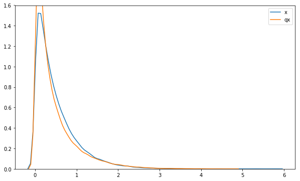

Gradient-based Monte Carlo. Consider an Empirical approximation with 1000 samples and use the algorithm ed.HMC.

from edward.models import Empirical

qx = Empirical(params=tf.get_variable("qx/params", [1000]))

inference = ed.HMC({x: qx})
inference.run(step_size=0.8)

Gamma and Empirical have unequal support so Gamma is transformed to the unconstrained space; by implementation, discrete delta distributions such as Empirical and PointMass are not transformed. ed.HMC then simulates Hamiltonian dynamics and writes the unconstrained samples to the empirical distribution.

In order to obtain the approximation on the original (constrained) support, we again take the inverse of the target distribution’s transformation.

from tensorflow.contrib.distributions import bijectors

x_unconstrained = inference.transformations[x]  # transformed prior
x_transform = x_unconstrained.bijector  # transformed prior's transformation
qx_constrained = Empirical(params=x_transform.inverse(qx.params))

Unlike variational inference, we don’t use ed.transform to obtain the constrained approximation, as it only applies to continuous distributions. Instead, we define a new Empirical distribution whose parameters (samples) are given by transforming all samples stored in the unconstrained approximation.

We can visualize the densities of the distributions. The figure below indicates that the samples accurately fit the Gamma distribution up to simulation error.

sns.distplot(x.sample(50000).eval(), hist=False, label='x')
sns.distplot(qx_constrained.sample(100000).eval(), hist=False, label='qx')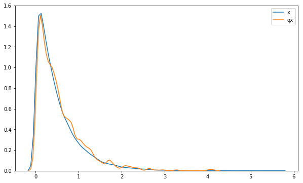

Acknowledgements & Remarks

Automated transformations have largely been popularized by Stan for Hamiltonian Monte Carlo (Carpenter et al., 2016). This design is inspired by Stan’s. However, a key distinction is that Edward provides users the ability to wield transformations and more flexibly manipulate results in both the original (constrained) and inferred (unconstrained) space.

Automated transformations are also core to the algorithm automatic differentiation variational inference (Kucukelbir, Tran, Ranganath, Gelman, & Blei, 2017), which allows it to select a default variational family of normal distributions. However, note the automated transformation from non-negative to reals in Edward is not \(\log\), which is used in Stan; rather, Edward uses \(\textrm{softplus}\) which is more numerically stable (see also Kucukelbir et al. (2017 Fig. 9)).

Finally, note that not all inference algorithms use or even need automated transformations. ed.Gibbs, moment matching with EP using Edward’s conjugacy, and ed.KLqp with score function gradients all perform inference on the original latent variable space. Point estimation such as ed.MAP also use the original latent variable space and only requires a constrained transformation on unconstrained free parameters. Model parameter estimation such as ed.GANInference do not even perform inference over latent variables.

References

Carpenter, B., Gelman, A., Hoffman, M. D., Lee, D., Goodrich, B., Betancourt, M., … Riddell, A. (2016). Stan: A probabilistic programming language. Journal of Statistical Software.
Casella, G., & Berger, R. L. (2002). Statistical inference (Vol. 2). Duxbury Pacific Grove, CA.
Kucukelbir, A., Tran, D., Ranganath, R., Gelman, A., & Blei, D. M. (2017). Automatic Differentiation Variational Inference. Journal of Machine Learning Research, 18, 1–45.